Antimony is an open-source, relying on graph composition where nodes represent primatives, 2d shapes, and loads of customizable operations and functions. The graph has an GUI akin to Grasshopper, the infamous Rhinoceros plugin. Antimony's interface includes a 3d viewport which has limited modeling capabilities that automatically log into the graph and a script editor. The script editor enables customization of all the graph nodes and is going to require more time for me to grasp. The advantage here is the algorithmic nature of the modeling. Changes can easily be applied throughout the entire history of the graph and propagate throughout the system. This way a decision made early in the modeling can be adjusted according to new information without breaking the series of subsequent decisions. Design versioning is fast. For me, there are a couple of limitations. One, the scripting interface is a hurdle, at this point, simply due to a lack of education on the subject. Two, Antimony in its basic form works with obstensibly with solid primitives; meaning, custom shapes requires to step back to limitation number one.
I jumped in, downloaded the free DMG build and found this five minute introductory tutorial which was plenty to get me going on the graph and viewport portions of the modeler.
Antimony screencast from Matt Keeter on Vimeo.
There are a few basic interfaces I will list here to save you time.
  Rotate...................Left Mouse
  Pan......................Right Mouse
  Quick Action menu........Shift[Key] A
Here is a screenshot from my own computer after completing the tutorial. #BaBoom.
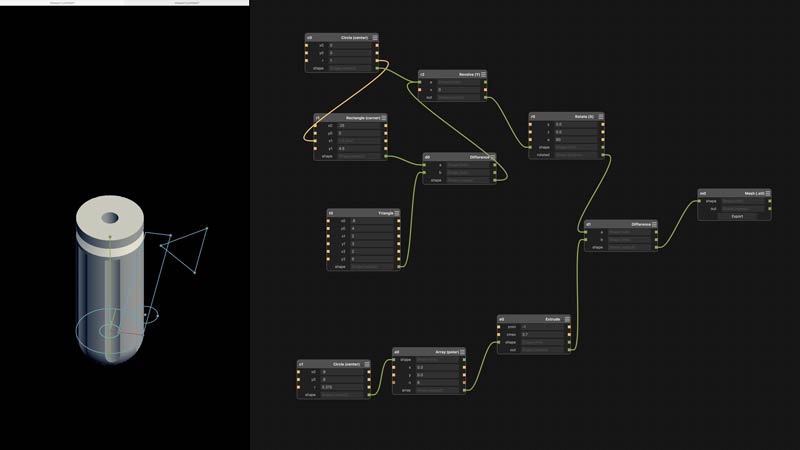
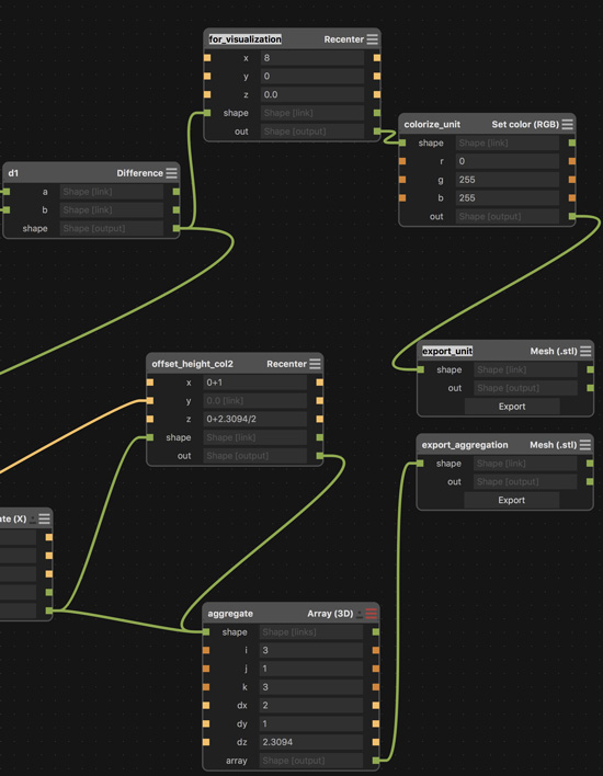
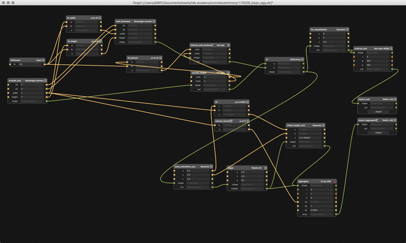
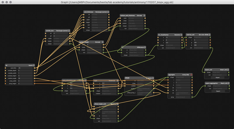
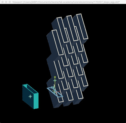
Alright now, lets get cracking. I built a basic unit and aggregation possibility for my final project. In reality, its early in development, but I imagine the final project to take on a more shapely appearance. However, that would require greater familiarity with the modeler and this version works well as a base. Further, I assume formal complexity may be adapted to the model over time. Feel free to do whatever you please with this:
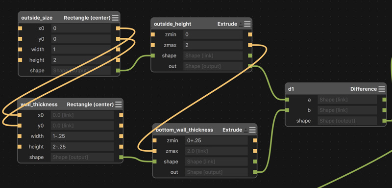
I will break it down. The unit is a rectangle with one side open. I started with two rectangle primitives, one for the outside dimensions and one to set the wall thickness. The "x0" and "y0" values are to set the origin of the center point of the rectangle. I need the thickness and outside rectangle to have the same center point, so the outputs of one are linked to the inputs of the other. Btw, in case of this model, all dimensions are relative. Straight away, it would be preferable to set the wall thickness in an equation: the output of the outside size into a thickness node that then spits the proper inside rectangle size to the wall_thickness node. That way I could simply update the outside size or the thickness value, rather than having to adjust each value in this current setup. In this model it is not a big deal; although, with added graph complexity labor increases exponentially. Next, the two shapes are extruded and the thickness of the bottom wall set by adjusting the "zmin" value of the thickness node. That will move the bottom of the primitive up the z-axis. For the hole in the top, the "zmax" of the thickness node should be at least equal to the outside height, thus the output of the outside height value is linked to the thickness node (a change in the overall height will automatically adjust the thickness so the unit will always be open at the top). In the graph, I was able to set these as simple equations because: math. The final step to get the unit is to difference the thickness from the outside primitive. Booleans are built into the CSG menu. "a" is the primary shape, "b" is the subtracting shape.
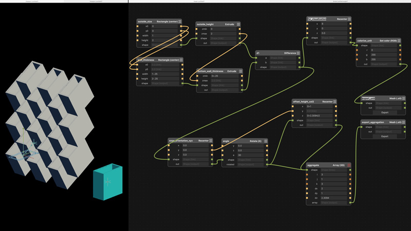
The next step is to aggregate the units. First, to make subsequent calculations simpler, I recentered the unit to the origin of the grid: 0,0,0. Then, rotate the unit on the X-axis some value. Finally, array the unit. The array node is split into values for quantity: i,j,k corresponding to direction: x,y,z. Again, equations would be useful here. "dx" equals outside width multiplied by 2 (offset two columns). "dz" is more complicated. I will explain below. Because the even number columns are offset on the z-axis, the rotated output was split to a recenter node to move an initial unit into position for arraying. The recentered node can connect into the same aggregate input.
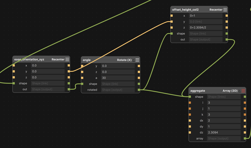
I used another 2D CAD application to find the "dz" value by sketching the system to scale in elevation. In this case, a 2x2 unit rotate 30 degrees copied along a vertical line to an intersection point on the outside wall. Again, this operation should be capable of using an equation based on the outside dimensions and the rotation angle; it is beyond my ability tonight. The found value is copied into the array node and divided in half for the second recenter node.
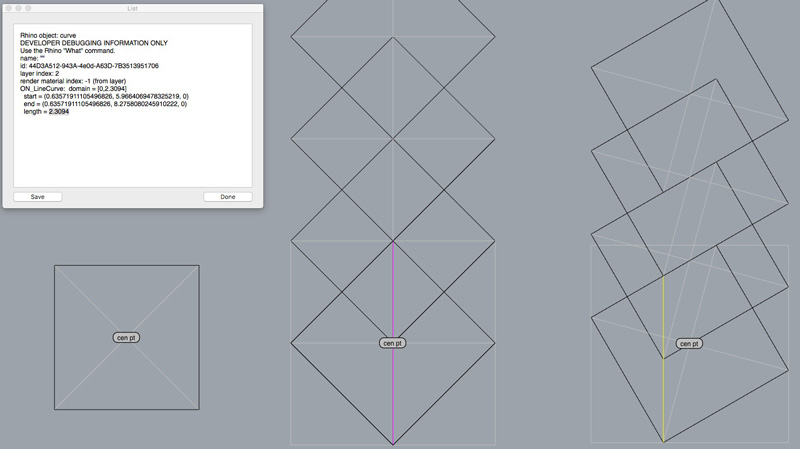
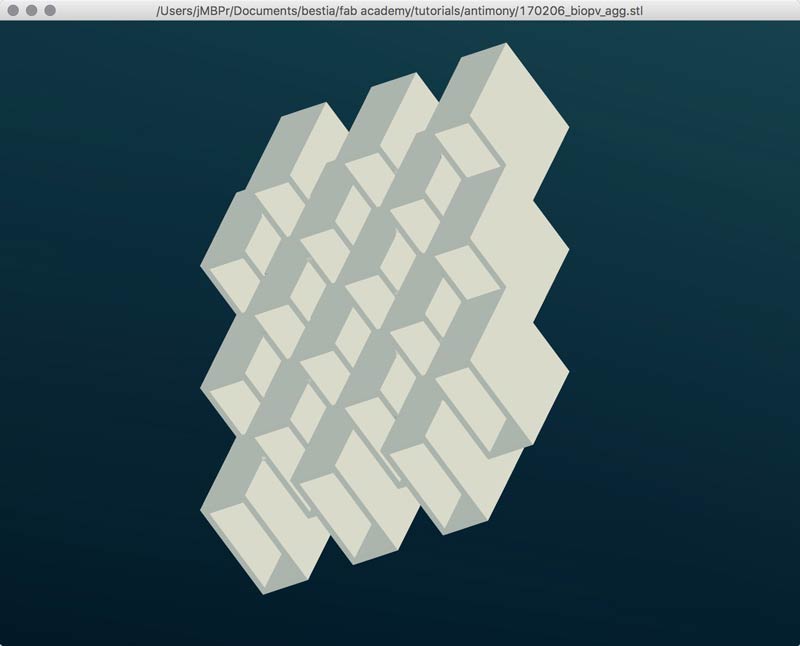
Finally, built into Antimony is an STL export node. Plug a shape output into the export shape input, use the defaults and push out an STL file. The second image is the STL opened in FSTL, another free application from Matt Keeter. I do not know why it rotates the output 180 degrees on the Y axis.
Update: Aside from the geometrical problem of solving for distance of array along the z-axis relative to the unit's rotation along the x-axis, many of the other missing bits of automation I solved. You can add a simple script node and click on the upper right corner to edit it. I was mistakingly adding an equal sign in the output line. Do not do that. Do this:
  output('y',y=w-th).......wrong
  output('y', w-th)........ding!
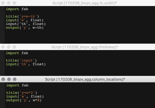
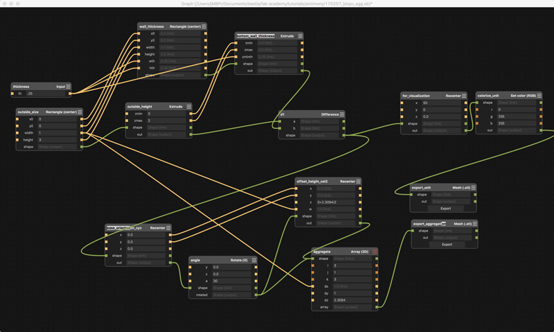
Looking at this, it appears yet inefficient. Although, it is operational. I believe I could edit the script in the thickness nodes to incorporate the now external formulas... And with the magic timelessness of the internet, success! Simply taking what I learned with the simple scripts one step forward, I could understand the preset scripts in the nodes and add some inputs and make little modifications to the formulas. In other words, customizing generic commands for specific needs. That is the whole point, right? The graph screen, before and after.
Here is an example of one of the thickness nodes with the previously external scripting nodes incorporated. I added two width inputs, for no other reason than a future option. Those inputs were sourced from the output of my thickness input node. That number shows up several times so it is simplest to set one controlling node. In fact, in the future, that node could have three thickness values for each of the axes. Aside from the added inputs, in the min & max formulas, I adjusted the height and width values for thickness as so:
  xmin, xmax = x0 - (width-wth)/2, x0 + (width-wth)/2
  ymin, ymax = y0 - (height-hth)/2, y0 + (height-hth)/2
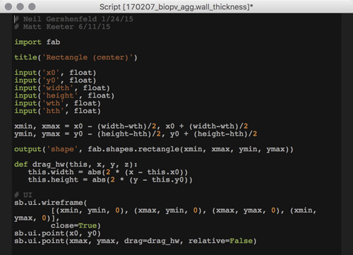
Adjusting the overall size along the X and Y axes and the wall thickness is now very easy. Now if I could only solve the geomtry problem for the array Z distance...
Update 2: As I was lying down for a nap, high school geometry came gushing from the depths of my suppressed memories. I was thinking of the Z-Array distance problem as a constrained CAD artist (find the intersection). When thought of as triangles, the solution is clearly a cosine formula. Reviewing this previous drawing, one angle is always square and one I set. Further, the length of the outside side, or height of the unit is set.
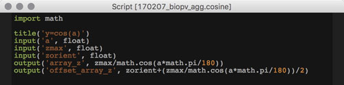
Now, write the math into a node. There are a few tricks to this. One, any script required in the outputs needs to be imported into the node. In this case, I need a cosine function, so "import math". In previous node screenshots in this post, "import fab" was called out; that was unnecessary. The cosine function requires radians so conversion math was added. Solving the hypotenuse, or yellow or pink line in the previous drawing, required this bit of code:
  output('array_z', zmax/math.cos(a*math.pi/180))
  zmax.....................unit outside height
  a........................rotation angle on X axis
  math.cos.................cosine script
  math.pi..................Π !
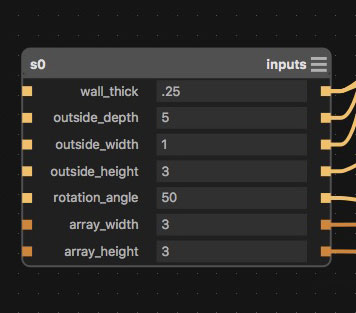
To simplify the interface, I made a master inputs node containing all the user-defined variables. Any change in this node propagates through the entire system and updates the model accordingly. And, finally, one screenshot of the final graph and one of the more attractive configurations I found after gleefully swapping numbers around for the last fifteen minutes.
I will post links to resources I have found helpful here.
- Antimony introduction : From Matt Keeter's blog.
- Very fast STL viewer : Download link. Also written by Matt Keeter.
- Antimony screencast : A brief introductory tutorial by Matt Keeter (building a screwdriver handle).
- Antimony : Download link.
- Antimony quick user's guide.
- Introducing Antimony... : An interview with Matt Keeter.
- Angle conversions : Little introduction to converting angles from degrees to radians and the other way too.
- Project file : My Antimony project file.
Share this post...
« Previous post :: History : Early concepts
2017.2.1 My ambition is to make an energy harvesting system using biological photovoltaics as an exhibition work to bring attention to clean, sensational possibilites for sourcing energy and the fact that we need [wildness] nature more than it needs humans. This system will be a network of modular components. Each module consists of a fabricated shell, preferrably from cradle-to-cradle capable materials, biological material (plant or algae, tbd), energy harvesting materials, bio-support materials. The network is connected to an energy storage and MCU. The MCU can be used for monitoring illuminance, humidity, temperature and volt output statistics to be used in...
Next post :: Cascading Style Sheets : CSS »
CSS describes how HTML elements are displayed. Because one piece of CSS code can alter the behavior of all of any single HTML element throughout all the pages of one website (or even multiple websites), writing CSS can save loads of time and effort customizing appearances. CSS can add background images or color, borders, change font attributes such as: style, color, and/or typeface, set margins, adjust website sizes for different devices, create image galleries, all sorts of great stuff. This is CSS: selector { declaration: value; } Or from the version of this website dated 2017.2.21: body { font-family: 'courier...